
Deprecated: Creation of dynamic property FusionSC_Column::$is_nested is deprecated in /home/mherbold/public_html/bravearmy.com/wp-content/plugins/fusion-builder/inc/class-fusion-column-element.php on line 553
Deprecated: Creation of dynamic property FusionSC_FusionText::$params is deprecated in /home/mherbold/public_html/bravearmy.com/wp-content/plugins/fusion-builder/shortcodes/fusion-text.php on line 127
My fellow Arthlings!
Over the past couple of weeks, I have been working on the planet generator for this Starflight remake. As many of you will know, the planet generator for the original game was one of their proudest moments. Inside the cover of the original Starflight box, there is a blurb about their planet builder:
About nine months after we started the actual programming, we came up with the idea for the fractal generator. A fractal generator so powerful that it could create surfaces in space. It took 6 man-years to create the technology, but it gave us the ability to cram 800 complex and unique planets into each game, instead of the 50 we’d had before. There are so many that even we haven’t explored them all.
On the back of the box, you will also note that they say it took 15 man-years to create the entire game. If you do the math, this means a full 40% of the entire development time was spent on just creating this fractal planet generator for the original game.
So, as not to insult the spirit of this game, I decided to dedicate a lot of time into also creating a fractal planet generator for this remake. And lo and behold, here it is!
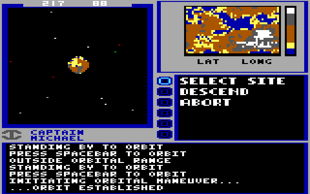
The generator starts with the original color and key of the planet. The color and key are grabbed from screenshots taken while in orbit around the planet and the Captain > Land menu item is selected.
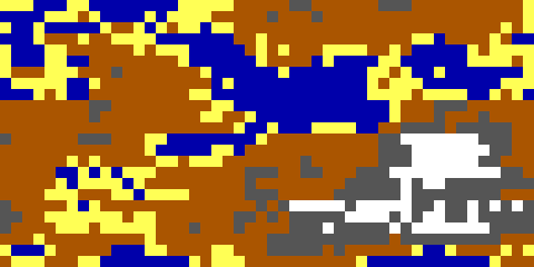
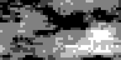
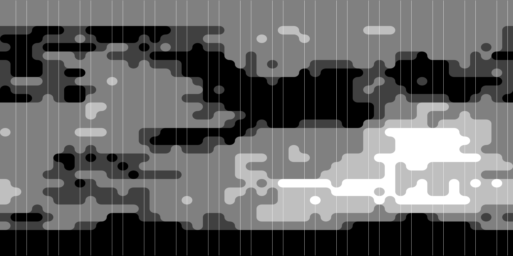
The first image is the original color extracted from the screenshot, and the second image is the height map extrapolated from the color key in the screenshot. These images are 48 by 24 in size. Not a lot of detail!
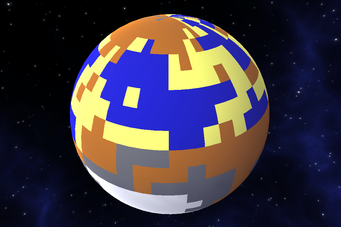
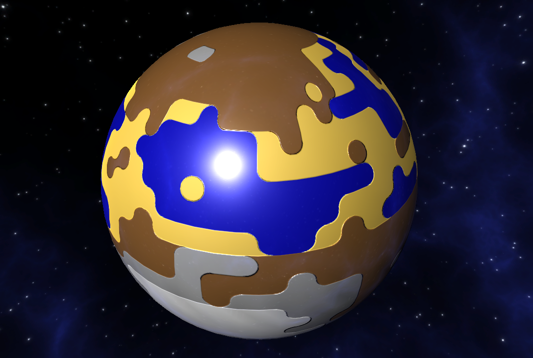
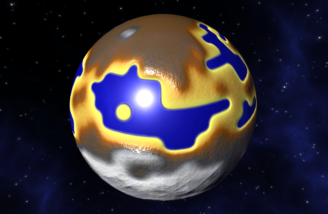
The next image shows what our 3D planet would look like with the original color map applied to it, without any modification.
Step 1 – Padding
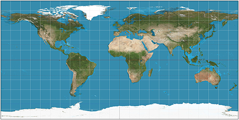
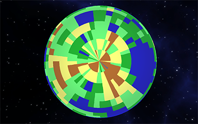
The first step is to add some padding to the top and bottom (North and South) of the original color maps. Why? Because these maps are supposed to be equirectangular maps that are applied to a spherical object. Let’s take a look at a real equirectangular map (see first image below). Notice the North and South ends of the map are stretched out horizontally. The white snow of Antarctica stretches all the way from the West end to the East end of the map. This is because those ends of the map actually correspond to a single point on the globe! So, what happens if we have multiple colors on those ends of the map? You get pole pinching (see the second image).
To avoid pinched poles, we add some padding to the top and bottom of the original map. What we pad the top and bottom with are selected by determining what the most used colors at the poles are. Here is the result – compare it with the original height map. I add 3 rows of padding on each side, making the map now 48 by 30 in size.

Step 2 – Contours
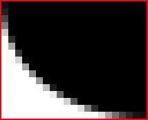
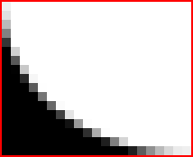
The next step is to increase the size and resolution of this height map. I have decided to implement a routine that I call “contours” generation. What it does is it sub-divides each pixel in the original color map into 2 by 2, and then each sub-pixel is replaced by either an “outside corner,” or an “inside corner,” or a “solid corner” tile based on the 3 by 3 pattern for each sub-pixel. The following images are the inside and outside corner tile images. The solid corner is just a solid fill. Note that these tiles are 21 by 17 in resolution. The reason is explained below.
Our target map resolution is 2048 by 1024. Since our height map currently has a resolution of 48 by 30, this means we need to scale up by a factor of 42 by 34. This will make the contours map 2016 by 1020. Since each pixel in the original map is subdivided into 2 by 2, this means each tile needs to be half the size of the scale factor, meaning they need to be 21 by 17 each. The following image shows the result of the contours generation step.

Step 3 – Scale to Power of Two
Now that’s looking a lot better already. For the next step, we need to scale that image up a little bit more so that it is truly 2048 by 1024. The naive approach is to just use bilinear filtering to scale it up. While that will work, it will blur the image just a tad bit. We want to keep this image as crisp as possible. So, instead of using bilinear filtering to scale the image up, I pad the top and bottom with rows of the same elevation value as used in step 2. That takes our vertical resolution from 1020 to 1024 by adding 4 rows. For the horizontal scaling, I duplicate some columns. I very cleverly select only columns that are on the centerline of each 2×2 tile to duplicate. That avoids duplicating edges, which would be very noticeable. The first image below is the result. I bet you can’t tell the difference between that image and the one above. The second image below indicates which columns I selected to duplicate (click on it to zoom in). The third image shows what a 3D rendering of the planet looks like now.

Step 4 – Blur Pass
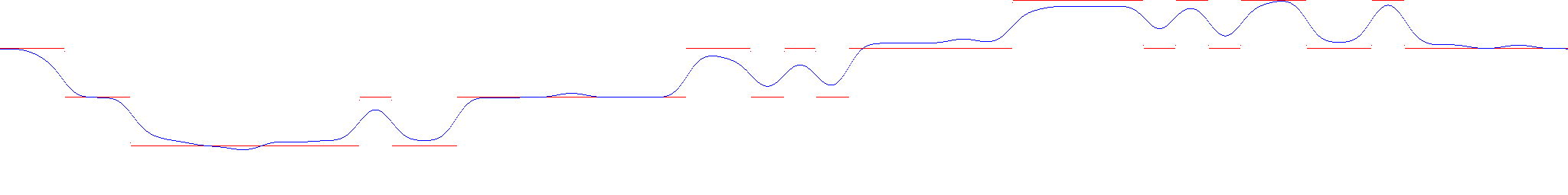
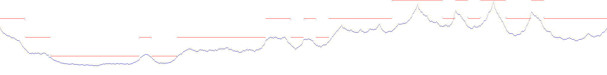
Now that we have a clean elevation map with a power of two horizontal and vertical resolution, it’s time to start doing some really interesting things to it. The first thing I do to it is to use a Gaussian blur filter to blur the elevation map. I blur it twice, first with a large blur kernel, and then with a smaller kernel. In between the two blurs, I reset the elevation to zero, where there is water. This gets me nice big blurs where the mountains should be, and a smaller blur to blend land into water (beaches). The first image below shows the result of the two blur passes. The second image shows an elevation profile, with the red line indicating the original elevation profile, and the blue line indicating the new elevation profile after the blur is complete. The third image shows what a 3D rendering of the planet looks like now.

Step 5 – Mountains and Hills
Now that we have a nice smooth elevation map, it is time to add some details. We want mountains in the higher elevations and hills in the lower and middle elevations. To do this, I apply some fractal noise. For the mountains, I use the “ridged” variation of Perlin noise, and for hills, I use standard Perlin noise. The first image shows the new elevation map after this process has been applied, and the second image shows the new elevation profile. The third image shows what a 3D rendering of the planet looks like now.

Step 6 – Hydraulic Erosion
Most people would be content with what has been done so far. Not me! Remember, the original crew spent six man-years developing the original fractal planet generator. SIX! Surely, I can spend a few more hours on this. So… bring in the hydraulic erosion machine! What is hydraulic erosion? It’s just a fancy way of saying soil erosion due to moving liquids (like rain). The problem with using a fractal noise generator to create mountains and hills is that they do not account for the millions of years of soil erosion from rain. Rain carves channels and rivers into solid granite rock. Rain gave us the grand canyon. And so, rain will give us beautiful worlds for this Starflight remake.
I made it rain, the likes that have not been seen since the days of Noah. Two million, 97 thousand, and 152 drops of rain each planet to be exact; one for each grid point on the elevation map. Each drop of rain is tracked as it hits the terrain and makes it way down to lower elevations. As the raindrop meanders throughout the elevation map, sediment is absorbed and deposited along the way. The full details of how this process works are too much for this blog, but you can find them in the code in Github.
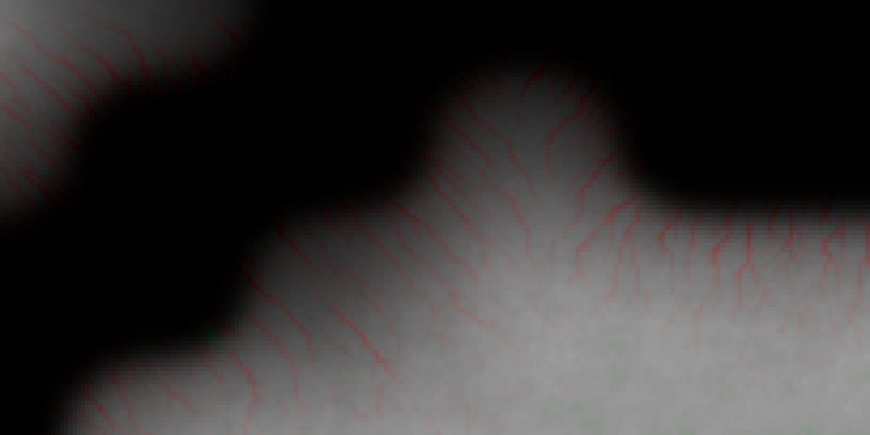
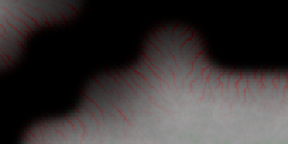
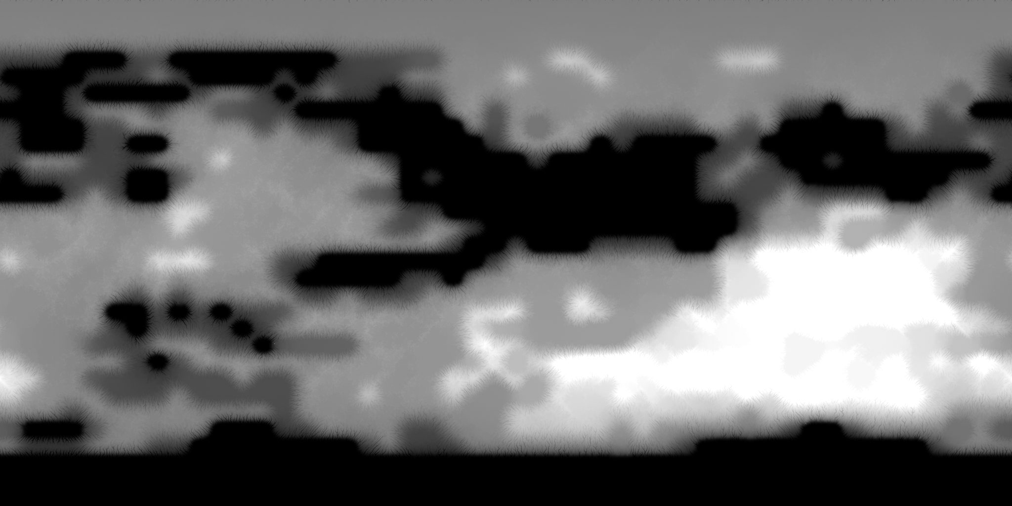
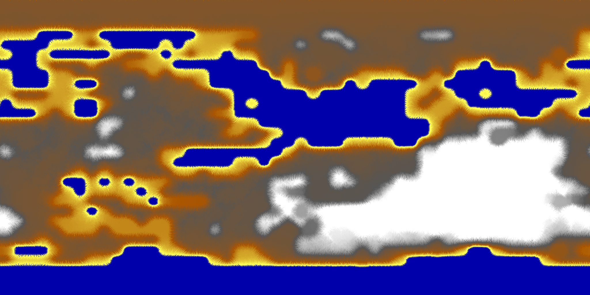
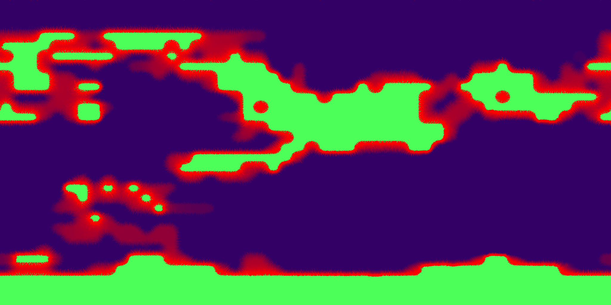
The following images show the changes in the terrain after some rain. The red areas indicate where sediment has been removed from the terrain. The green areas indicate where sediment has been added to the terrain. The first image shows changes after about 65,000 drops of rain. The second image shows changes after about 1 million drops of rain. The final image shows changes after all 2,097,152 drops of rain have been processed.

The next image shows what the terrain height map now looks like. Click on it to zoom in and see the details.
Step 7 – Albedo Pass
For our next trick, we will convert the terrain height map into colors. We do this by using a massaged version of the color key of the map from the original game. This is a pretty straightforward process. The image below shows the result.
Step 8 – Effects Pass
Now it is time to create the effects texture map. What is an effects texture map? In our case, it is a texture map where the red, green, and blue channels control the parameters of some special effects applied during the shading process. The red channel controls the “roughness” of the terrain. The rougher the terrain is, the duller the specular shine will be. The green channel controls where “water” appears on the map. This channel is used to mask out where the animated water waves will be rendered. And then finally, the blue channel controls the “reflectivity” of the terrain. Water is where the terrain is most reflective – and this channel is somewhat related to the red (“roughness”) channel. The image below shows the effects map.
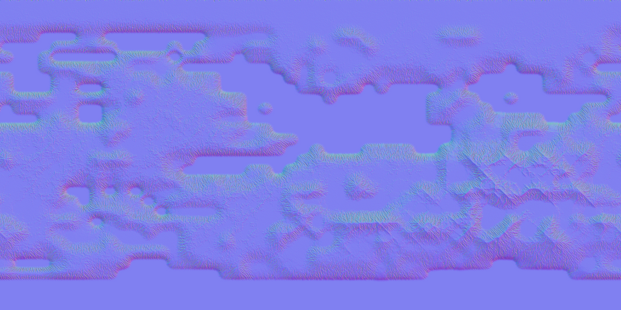
Step 9 – Normals Pass
Everything looks great so far, but we need to add one more texture map. This is called the “normal” map. It describes the facing direction of each point on the surface and affects all of the lighting calculations. The planet generator simply looks at each point on the map and compares its height with all of the surrounding points on the map, and figures out from that what direction that point on the surface is facing. The result is coded as a color map, but it is not actually color data. The colors are actually unit vectors, where the red, green, and blue channels represent the X, Y, and Z components of the vector. Here is the normal map image.
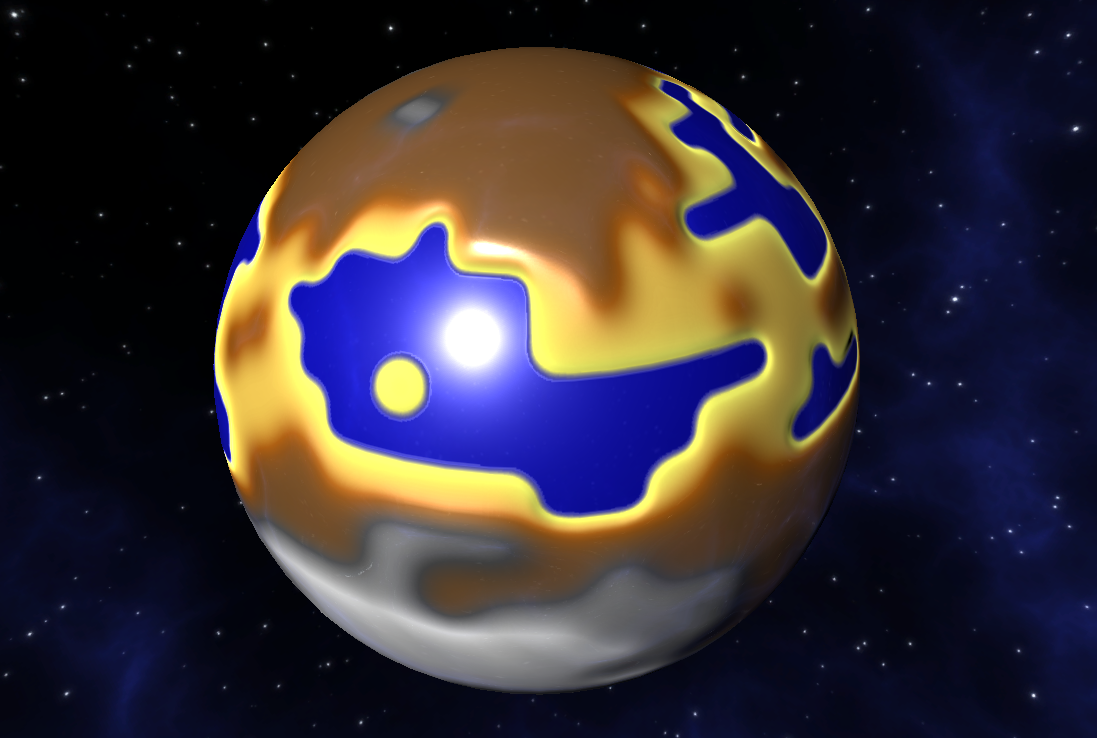
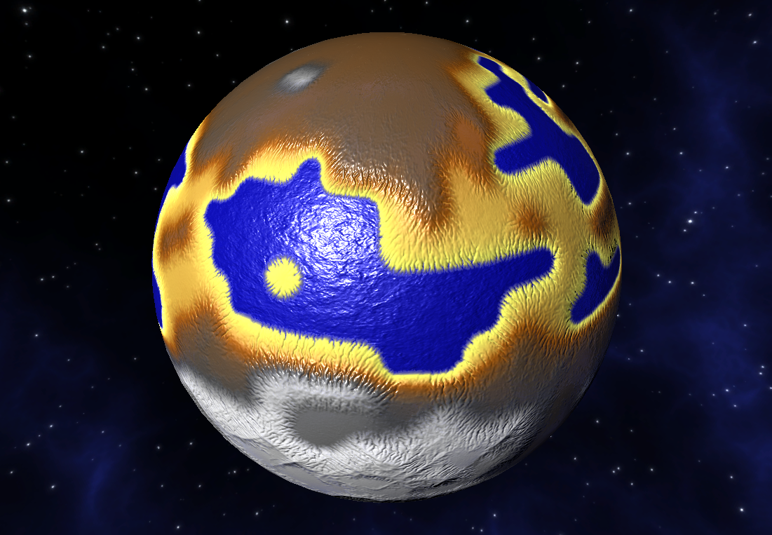
The Final Result
Put it all together, and this is what we have.
I have implemented multi-threaded processing for most of the steps of the planet generator. Even with everything nicely threaded, it still takes up to 2 minutes to generate all of the texture maps on my 10-core Area-51 Alienware machine. Do the math – 811 planets x 2 minutes = a little more than 24 hours to generate texture maps for every planet in the game. But really it will be far less than this, as I plan to have a completely different (and much faster) process for gas giants.
Very impressive and thanks for putting so much work into such a great remake.
Brilliant!!!!